Introduction
ARIMA (AutoRegressive Integrated Moving Average) is a widely used statistical method for time series forecasting. It combines autoregression (AR), differencing (I), and moving average (MA) components to model and predict future values in a time series. In this article, we will explore how to use ARIMA to forecast financial data, such as stock prices or exchange rates, using R.
What is ARIMA?
ARIMA models are defined by three parameters: p, d, and q.
-p (AR - AutoRegressive): The number of lag observations in the model.
-d (I - Integrated): The number of times the data is differenced to make it stationary.
-q (MA - Moving Average): The size of the moving average window.
The general form of an ARIMA model is ARIMA(p,d,q).
Steps for ARIMA Forecasting
- Load and Prepare the Data: Import the financial time series data and ensure it is in a suitable format.
- Check for Stationarity: Use statistical tests or visual inspection to determine if the data is stationary. If not, apply differencing.
- Select ARIMA parameters: Use tools like ACF (Autocorrelation Function) and PACF (Partial Autocorrelation Function) to identify p and q. Determiner d based on the number of differencing steps required.
- Fit the ARIMA model: Use the identified parameters to fit the ARIMA model to the data.
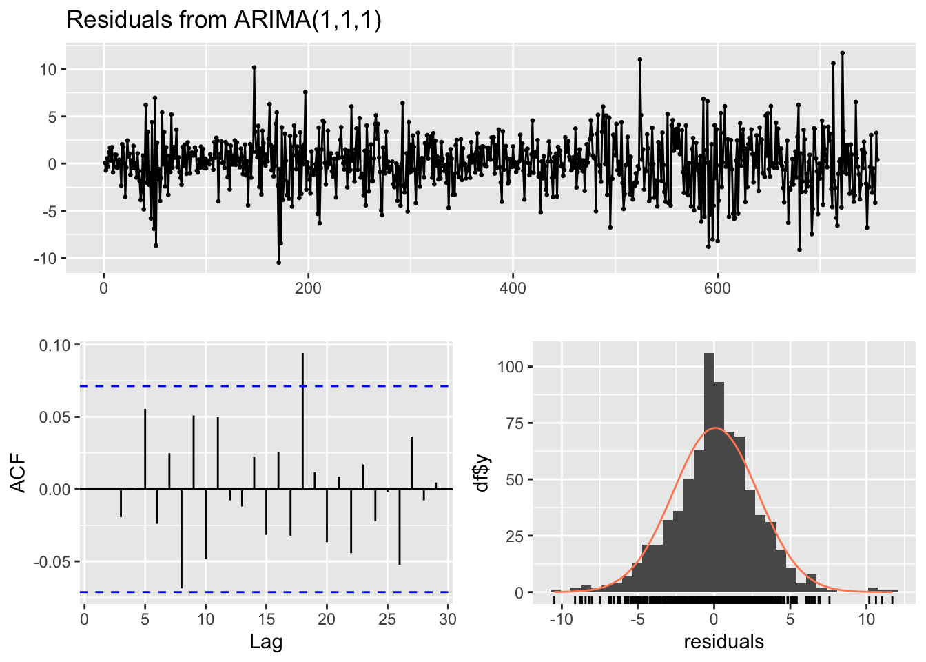
- Validate the Model: Check the residuals to ensure they resemble white noise.
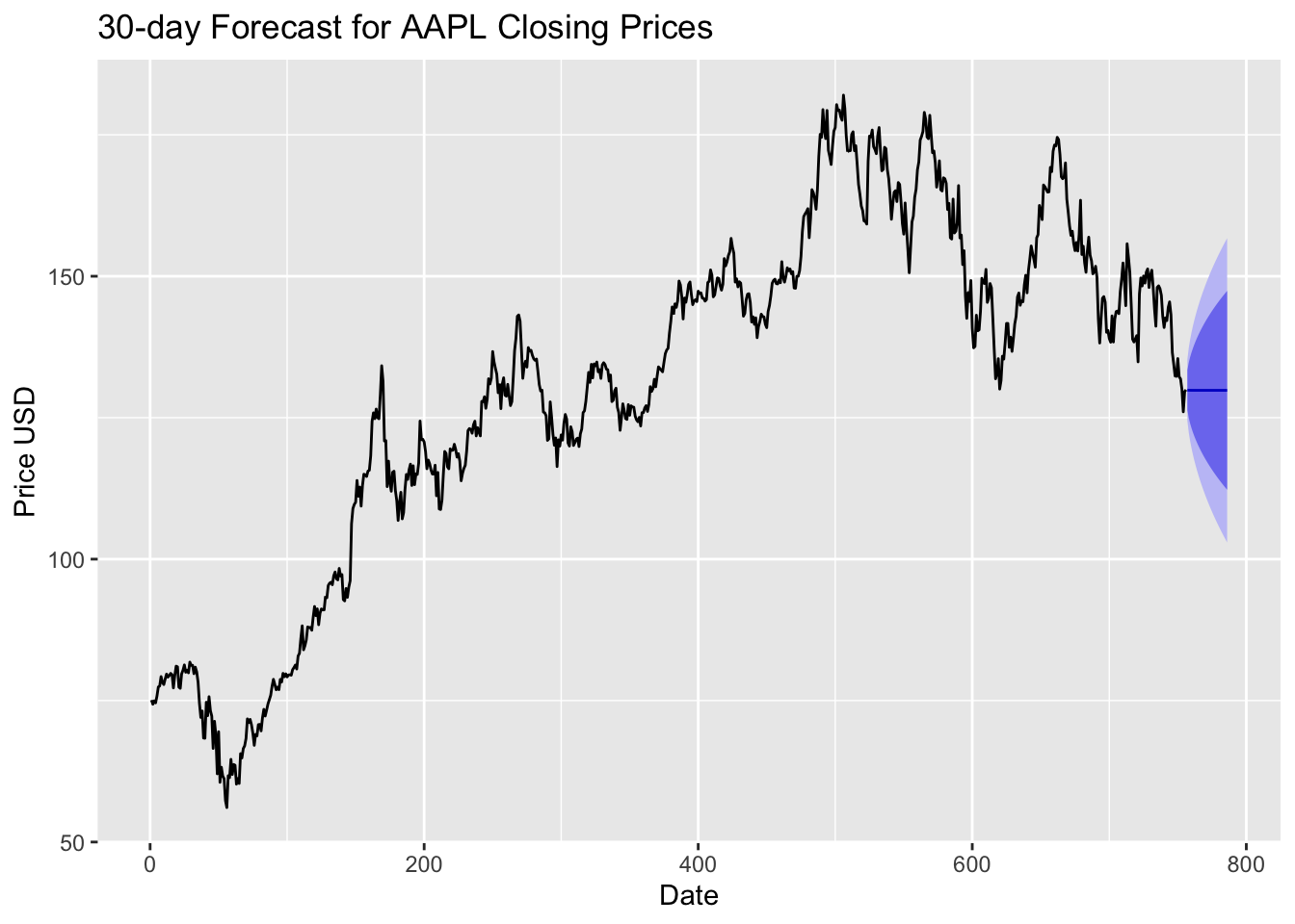
- Forecast: Use the fitted model to predict future values.
Example: Forecasting Stock Prices
Let’s walk through a simple example using the quantmod package to download stock data and the forecast package to fit an ARIMA model.
Step 1: Load Required Libraries and Data
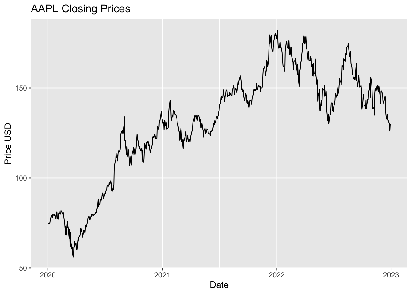
We start by loading necessary libraries and gathering the financial data we want to analyze, such as stock prices or exchange rates. This data is typicale organized by date and value (e.g., dialy closing prices).
Loading required package: xts
Loading required package: zoo
The following objects are masked from 'package:base':

    as.Date, as.Date.numeric
Loading required package: TTR
Registered S3 method overwritten by 'quantmod':
  method            from
  as.zoo.data.frame zoo
Setp 2: Check for Stationarity
Now we check if the data is “stationary”, which means its statistical properties (like mean and variance) don’t change over time. Financial data often has trends or patterns that make it non-stationary.
    Augmented Dickey-Fuller Test

data:  aapl_close
Dickey-Fuller = -1.2623, Lag order = 9, p-value = 0.8906
alternative hypothesis: stationary
If the data is not stationary, apply differencing:
Step 3: Identify ARIMA Parameters
We determine the values of p, d, and q for the ARIMA odel. These parameters control how the model looks at past data (p), how much differencing is applied (d), and how it smooths out noise (q).
Step 4: Fit the ARIMA model
With the selecte parameters we train the ARIMA model on our data. This step involves finding the best mathematical relationship between past and future values.
Call:
arima(x = aapl_close, order = c(1, 1, 1))

Coefficients:
         ar1      ma1
      0.3965  -0.4611
s.e.  0.3492   0.3372

sigma^2 estimated as 7.759:  log likelihood = -1844.76,  aic = 3695.52

Training set error measures:
                     ME     RMSE      MAE        MPE     MAPE      MASE
Training set 0.08120946 2.783715 2.069065 0.05190092 1.657774 0.9963087
                     ACF1
Training set 0.0003378316
Step 5: Validate the Model
The model’s performance can be checked by analyzing its errors (called residuals). Ideally, the errors should look like random noise, with no obvious patterns, ensuring that the model isn’t making systematic mistakes and is ready for real-world predictions.
    Ljung-Box test

data:  Residuals from ARIMA(1,1,1)
Q* = 10.945, df = 8, p-value = 0.2048

Model df: 2.   Total lags used: 10
Step 6: Forecast Future Prices
Finally, we use the trained model to predict future values. For example, the next 30 days.
Conclusion
ARIMA models are powerful tools for time series forecasting, especially in financial markets. By following the steps outlined above, you can model and predict stock prices or other financial data.
However, it’s important to remember that financial markets are influenced by many external factors, so ARIMA models should be used in conjunction with other analysis techniques.
Moving Forward
While ARIMA models are powerful for time series forecasting, there are several ways to extend and improve your analysis:
- Incorporate External Variables
ARIMA models are univariate, meaning they only use the target time series for forecasting. However, financial data is often influenced by external factors such as interest rates, economic indicators, or news events. Consider using SARIMAX (Seasonal ARIMA with Exogenous Variables) or other models like VAR (Vector Autoregression) to incorporate additional variables.
- Experiment with Seasonal ARIMA (SARIMA)
If your financial data exhibits seasonality (e.g., quarterly earnings reports), you can extend ARIMA to SARIMA by adding seasonal parameters (P, D, Q, m). This allows the model to capture recurring patterns in the data.
- Combine with Machine Learning Models
Hybrid models that combine ARIMA with machine learning techinques (e.g. Random Forests, Gradient Boosting, or Neural Networks) can often improve forecasting accuracy. For example, you can use ARIMA to model linear components and a machine learning model to capture non-linear patterns.
- Explote Alternative Time Series Models
While ARIMA is a popular choice, other models like GARCH (Generalized Autoregressive Conditional Heteroskedasticity) for volatility modeling, Prohpet for automated forecasting, or LSTM (Long Short-Term Memory) networks for deep learning-based approaches may be better suited for certain types of financial data.
- Perform Robust Model Evaluation
To ensure your model generalizes well, use techniques like cross-validation, rolling forecasts, or out-of-sample testing. Metrics such as Mean Absolute Error (MAE), Mean Squared Error (MSE), or Mean Absolute Percentage Error (MAPE) can help evaluate model performance.
- Consider Real-World Constraints
Financial markets are highly dynamic and influenced by unpredictable events (e.g., geopolitical developments, pandemics). Always complement statistical models with domain knowledge and qualitative analysis to make informe decisiones.